Welcome to Deep Learning Tutorial

Deep Learning

Contents

1 Purpose of this tutorial
2 Intro
3 Deep Learning and Neural Networks
4 Perceptron
5 Sigmoid neuron
6 Learning Algorithms
- 6.1 Gradient Descent

Purpose of this tutorial

In this tutorial I try to introduce the concepts of Deep Learning, Those who know the basics of programming can follow this tutorial and develop their own Deep Learning models for problem solving. I will start with the mathematics of Deep Learning which may look intimidating for a beginner. I would like to get the basics right and give you the intuition behind these algorithms and later get into the Matrix Calculus that is involved with Deep learning.

Intro

Deep Learning belongs to a set of Mathematical algorithms that are used to identify patterns in data. The data can be of any form like text, images, video, audio or any other form of metadata. The terms Deep learning, Machine Learning and Artificial Intelligence are used interchangeably but there are subtle differences among them.

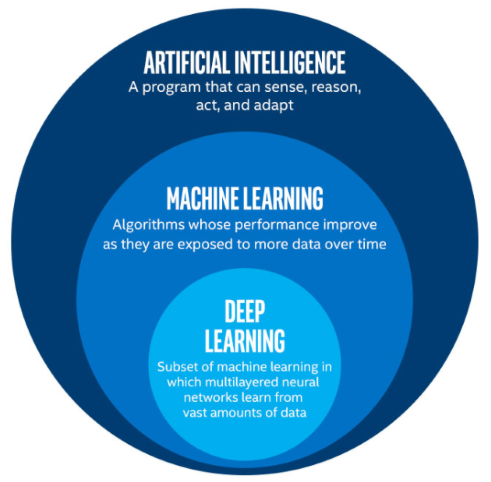
AI in terms of Computer science refers to the simulation of human intelligence in machines that are programmed to think like humans and mimic their actions. The term may also be applied to any machine that exhibits traits associated with a human mind such as learning and problem-solving. It is necessary to know that these problem solving traits are side effects of mathematical algorithms, that help computers learn the patterns for problem solving instead of programming them.

Machine Learning is a subset of AI (algorithms) and Deep Learning is a subset of Machine Learning Algorithms. The Deep Learning paradigm draws its inspiration from the workings of an animal brain, ie; it mimics the functionality of a group of neurons that are interconnected with each other in a layered structure.

Deep Learning and Neural Networks

We use Neural Networks to visualize deep learning algorithms as they are really good at abstracting the mathematical equations involved in Deep Learning. Neural networks is a collection of neurons that are organized in a layered fashion.

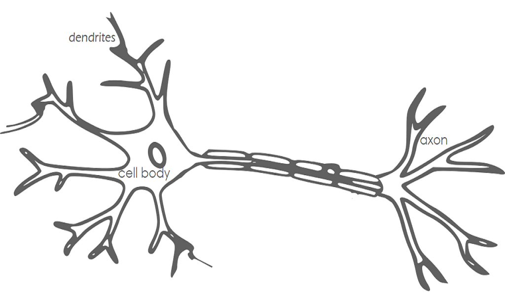
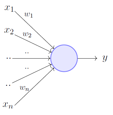
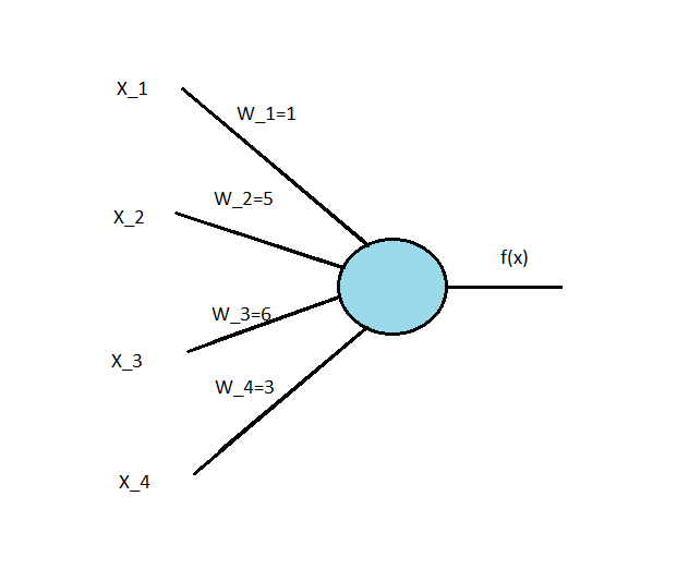
Each unit (shown in Fig 2 in the red box) is called a neuron. This neuron mimics the working of a neuron in an animal brain. Each neuron (animal neuron / mathematical neuron) takes the input signals, does some signal processing and generates an output signal that is dependent on (in mathematical terms a function of) the input given. This simple neuron (from here on we are referring to the mathematical one) can be used to solve basic mathematical problems and a network of these neurons can solve complex problems like detecting a face or deciding how to drive a car given enough number of neurons and enough computational power to run our model (which is not possible to program).

I am not just making these claims, we will see how this can be done in the sections ahead.

Perceptron

This concept was first introduced in 1958 by Frank Rosenbaltt. Perceptron is a Neural Network in its simplest form. It consists of a single neuron which takes $n$ binary inputs and $n$ weights which are associated with each of them, weights represent the importance of each input. The perceptron produces a binary output $f(x) \in \{0,1\}$ . The output $f(x)$ is dependent on the threshold value, $w^T x$ (it is a parameter of the perceptron). It can be represented as,

$f(x) = 1$ if $W^T X > 0$ & $0$ if $W^T X \leq 0$

Note that the wieghts $w$ and inputs $x$ are represented as vectors in the above equation where,

$W=\{w_1, w_2, ... , w_n | w_i \in {\rm I\!R} \}$ and $X=\{x_1, x_2, ... ,x_n | x_i\in \{0,1\}\}$

Fig 5: Graphical representation of a perceptron

In Fig 5, the region colored in red represents the vector space $f(x)> 0$ and the blue region represents $f(x)\leq0$ . The boundary between the two regions is the perceptron boundary $f(x)=W^T X$ that is a function of inputs and the perceptron parameter $w$ associated with each input.

Perceptron acts as a binary classifier, in other words it can classify the input elements into 2 groups and this classification is based on the parameter $w$ , which is learned by the perceptron model by iterating over the input data $X$ until it can land on some vales of $W$ that is able to classify the input into one of the 2 classes.

Let us consider surfing, for example. If you want to develop a perceptron which can tell you whether the conditions are favorable for surfing. Let us first consider the factors that dictate the surfing conditions

Water temperature, $x_1$ {0: cold, 1: normal}
Waves, $x_2$ {0: erratic wavy conditions, 1: good wavy conditions}
Cyclone_warning, $x_3$ {0: no cyclone expected, 1: expected cyclone }
Shark_warning, $x_4$ {0: expecting sharks in the surfing area, 1: no sharks expected in the surfing area }

Now let us associate each input wit a corresponding weight value

Since water temperature is not as important compared to $x_3$ or $x_2$ we shall give it a weight value of $w_1=1$
Since it is dangerous to surf in erratic waves, we will give it a higher weight value, $w_2=4$
We will give a higher value for cyclone_warning as it is not advisable to surf in such conditions, $w_3=6$
Since sharks are not really as dangerous as wave conditions or cyclone_warning, since shark attacks are over exaggerated , we shall give it a moderate weight value, $w_4=3$

The output $f(x)$ defines if its favorable for surfing of not

If $f(x)= 0$ unfavorable conditions for surfing
if $f(x)=1$ favorable conditions for surfing

Now let us consider the case $x=[0,1,0,0]$ . It means that the water temperature is cold, there is a cyclone warning and sharks are expected in the surfing area. Now if we check with our classifier equation, we have

$W^T X = \begin{bmatrix} 0\\1\\0\\0\end{bmatrix} \begin{bmatrix}1&4&6&3\end{bmatrix} =4$

Since $W^T X > 0$ , $f(x)=1$ , indicating favourable conditions for surfing

As you can see that even with a cyclone warning, we got the classifier to predict favorable conditions for surfing, to fix such abnormalities in our models we usually have a second parameter called a bias $b$ . Therefore the new perceptron classifier can be written as

$f(x) = 1$ if $W^T X - b > 0$ & $0$ if $W^T X -b\leq 0$

or it can also be incorporated into the weight vector where $w_0=-b$ with $x_0=1$ , it will have the same effect. Let us check the classifier again, but this time including the bias value $b=4$

$W^T X = \begin{bmatrix} 1\\0\\1\\0\\0\end{bmatrix} \begin{bmatrix}-4&1&4&6&3\end{bmatrix} =0$

Since $W^T X \leq 0$ , $f(x)=0$

Now we have a decent perceptron model to check if conditions are favorable for surfing. let us take another case where $x=[1,1,0,0]$

$W^T X = \begin{bmatrix} 1\\1\\1\\0\\0\end{bmatrix} \begin{bmatrix}-4&1&4&6&3\end{bmatrix} =1$ , Since $W^T X > 0$ , $f(x)=1$ , We got favorable conditions for surfing.

Perceptrons can only classify linearly separable data. That is, if a straight line can be drawn through the vector space of the input data perceptron will be able to classify it. It will fail in the case of non linearly separable data. Another limitation of perceptron is that a small change in weights or bias can cause a large shift in the classifier. In other words it is very sensitive to changes in weights and biases.

Note that we have decided the weights for our perceptron. In reality, The perceptron has to learn the weights on it own. The Learning Algorithm does this, we shall discuss it in the further sections

$W^T X$ is called the dot product of weights and input vectors. It can also be written as $\sum_{i=0}^n w_i x_i$ . It is one and the same, just different notations. Perceptron can also be seen as an aggregate of weights and inputs, which is passed to an activation function. Step function, acts as an activation function in case of Perceptron.

Sigmoid neuron

Sigmoid neuron is also a simple neuron which helps us deal with the limitations of perceptrons. Like perceptron Sigmoid neuron is also a binary classifier but it is able to produce a non-linear classification, which is desirable because, in all most all of the real world applications we need a non-linear classifier. The sigmoid neuron can take inputs of range 0 to 1. Input, $X=\{x_1, x_2, ..., x_n| x_i \in[0,1]\}$ . So, 0.733 is an acceptable input value where as a perceptron can not accept such data. Weights can take any real values $W=\{w_1, w_2, ..., w_n | w_i \in {\rm I\!R} \}$ . The aggregate $W^T X$ is passed to an activation, which is a sigmoid function, $\sigma (.)$ . Sigmoid neuron can be represented as,

$f(x)= \sigma(W^T X)$ or $f(x)=\sigma(\sum_{i=0}^n w_i x_i)$

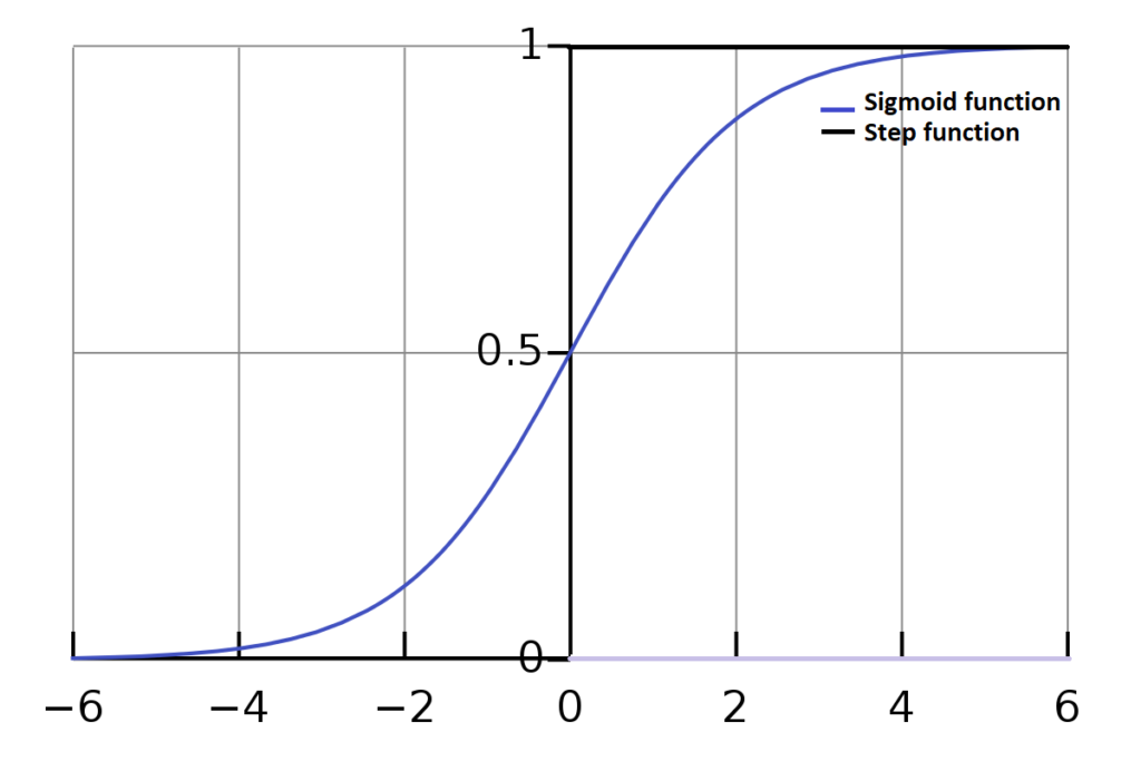
The sigmoid function is given by the equation, $\sigma(x)=\frac{1}{1+\exp{-x}}$ . Therefore, the output function of a sigmoid neuron is given by $f(x)=\frac{1}{1+\exp{-W^T X}}$

The sigmoid function has properties that help us overcome the limitations of the perceptron. First, It takes all vales from 0 to 1, which allows us to use any real valued data by normalizing it. . There are a wide variety of sigmoid functions, logistic function is widely used in deep learning, even hyperbolic tangent function ( $tanh(x)$ ) is used some times. Secondly, they have a smooth S shaped curve which increases monotonically, unlike the step function which abruptly changes its value.

Learning Algorithms

Gradient Descent

Further Sections will be uploaded on soon